To see the article headlines processed in this analysis, visit Articles Shared by Doppelgänger.
Building the Term Document Matrix
A Term Document Matrix (TDM) is a mathematical matrix that graphically represents the frequency of terms that occur in a collection of documents. In this matrix, rows correspond to terms and columns correspond to documents, or vice versa, depending on the structure chosen. Each cell in the matrix indicates the frequency of a term in a particular document.
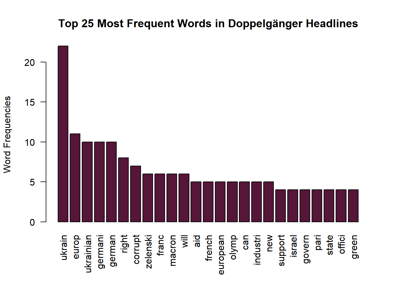
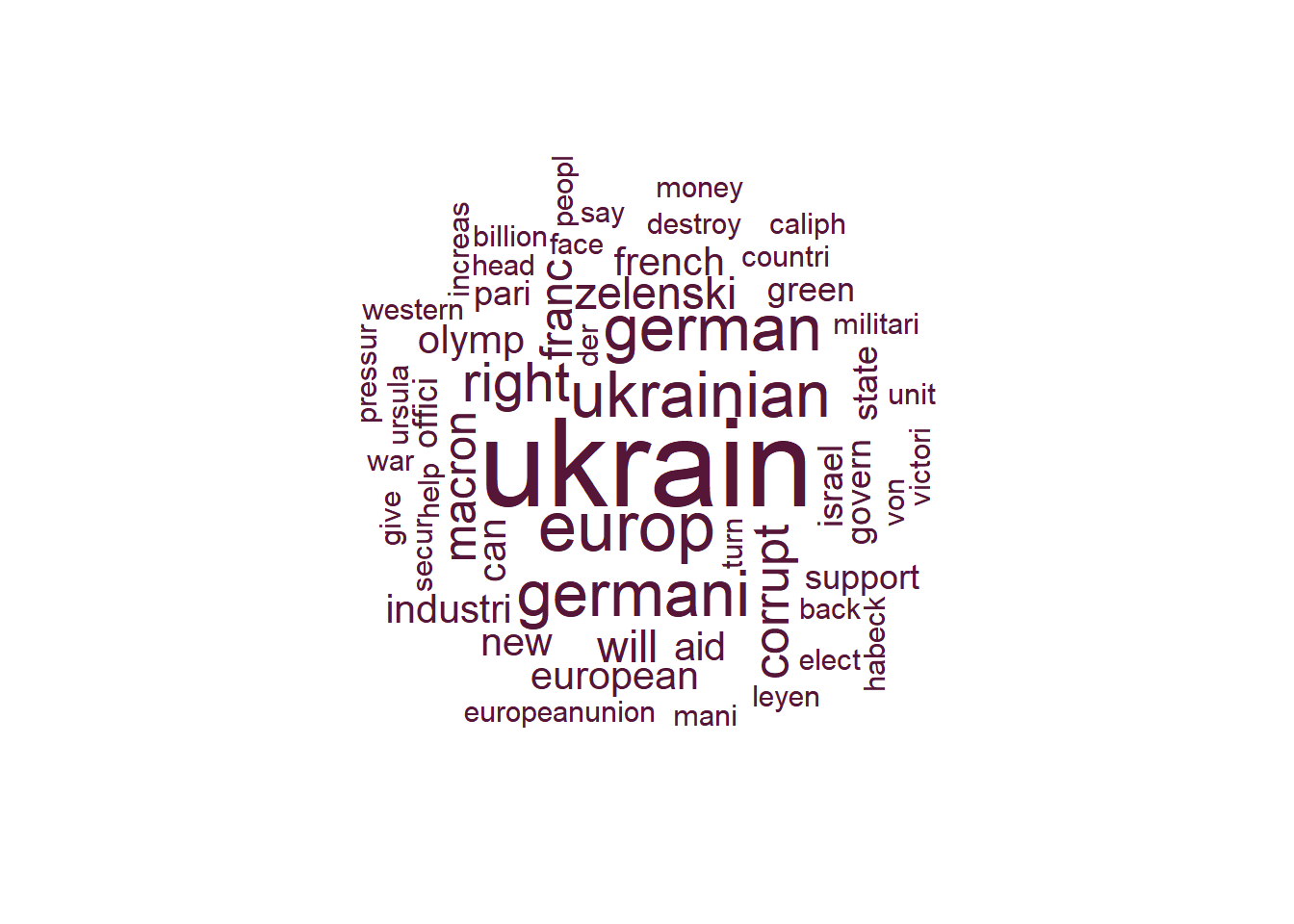
Visualizing the Most Common Words
Generate a Bar Chart
Generate the Word Cloud
Topic Modeling
Determine the ideal number of and identify topics.
     Topic 1   Topic 2     Topic 3    Topic 4
[1,] "ukrain"  "ukrainian" "europ"    "zelenski"
[2,] "aid"     "corrupt"   "ukrain"   "will"
[3,] "german"  "german"    "french"   "germani"
[4,] "support" "olymp"     "macron"   "right"
[5,] "countri" "pari"      "european" "ukrain"
Sentiment Analysis in R
Sentiments in texts can be classified as positive, neutral, or negative. They can also be quantified using a numerical scale to express the intensity of the sentiment.
Code
# Load necessary libraries
library(syuzhet)
library(ggplot2)
Sentiment Analysis using Syuzhet Method
Extract sentiment scores and view initial elements and summaries.
Code
# Calculate sentiments using the Syuzhet method
syuzhet_vector <- get_sentiment(text, method="syuzhet")
# Display first few entries of the sentiment scores
head(syuzhet_vector)
[1] 0.000000e+00 1.500000e+00 -2.775558e-17 5.000000e-01 -2.050000e+00
[6] 2.500000e-01Code
# Generate summary statistics for the Syuzhet sentiment scores
summary(syuzhet_vector)
Min. 1st Qu. Median Mean 3rd Qu. Max.
-2.0500 -0.7500 -0.1000 -0.1949 0.2750 2.5000 Sentiment Analysis using Bing Method
Apply the Bing method, inspect the first few entries, and summarize.
Code
# Calculate sentiments using the Bing method
bing_vector <- get_sentiment(text, method="bing")
# Display first few entries
head(bing_vector)
[1] 0 0 1 1 -2 -1Code
# Summary statistics
summary(bing_vector)
Min. 1st Qu. Median Mean 3rd Qu. Max.
-2.0000 -1.0000 0.0000 -0.3333 0.0000 2.0000 Sentiment Analysis using AFINN Method
Analysis with AFINN, examining initial outputs and summary statistics.
Code
# Calculate sentiments using the AFINN method
afinn_vector <- get_sentiment(text, method="afinn")
# Display first few entries
head(afinn_vector)
[1] 0 1 0 2 -2 -1Code
# Summary statistics
summary(afinn_vector)
Min. 1st Qu. Median Mean 3rd Qu. Max.
-7.0000 -2.0000 0.0000 -0.7143 0.0000 5.0000 Bing Method: This method utilizes a binary scale where:
- -1 represents negative sentiment
- +1 denotes positive sentiment
AFINN Method: This approach employs an integer scale ranging from:
- -5 (most negative)
- +5 (most positive)
Syuzhet Method: This technique employs the NRC emotion lexicon, which associates words with eight different emotions (anger, fear, anticipation, trust, surprise, sadness, joy, and disgust) and two sentiments (negative and positive). It provides a complex and nuanced understanding of emotional undertones in text data.
To effectively compare the sentiment analysis results from different methods, it’s important to normalize their outputs to a common scale because they use different rating systems. A practical approach in R for this standardization is to use the sign function, which adjusts the outputs as follows:
Converts all positive numbers to 1
Converts all negative numbers to -1
Keeps zero values unchanged as 0 This simplification allows for direct comparison across different sentiment analysis methods.
     [,1] [,2] [,3] [,4] [,5] [,6]
[1,]    0    1   -1    1   -1    1
[2,]    0    0    1    1   -1   -1
[3,]    0    1    0    1   -1   -1
Emotion Analysis
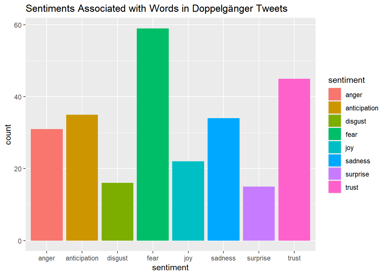
The NRC Word-Emotion Association Lexicon (EmoLex) facilitates the classification of words according to their association with various emotions and sentiments. EmoLex categorizes English words into eight distinct emotions (anger, fear, anticipation, trust, surprise, sadness, joy, and disgust) and two sentiments (negative and positive). Further details on EmoLex can be found on Saif Mohammad’s website.
The get_nrc_sentiments function generates a data frame where each row corresponds to a specific sentence from the analyzed text. This data frame has ten columns. Each column represents one of the eight emotions or one of the two sentiment valences.
   anger anticipation disgust fear joy sadness surprise trust negative positive
1      0            0       0    0   0       0        0     0        0        0
2      0            0       0    0   0       0        0     2        0        3
3      0            0       0    0   0       0        1     2        0        1
4      0            0       0    0   0       0        0     0        0        0
5      0            0       0    0   0       0        0     0        1        0
6      1            0       1    1   0       1        0     0        1        1
7      0            0       0    0   0       0        0     0        0        0
8      1            0       0    1   0       0        1     0        1        0
9      0            0       0    0   0       0        0     0        0        0
10     0            0       1    0   0       0        0     1        1        1
The next step is to create two plots charts to help visually analyze the emotions associated with the words in each headline.
To better understand the main emotions in the headlines, we can view these numbers as percentages that represent the share of key words falling under each sentiment category.
Citation
@article{infoepi_lab2024,
  author = {{InfoEpi Lab}},
  publisher = {Information Epidemiology Lab},
  title = {Sentiments and {Emotions} in {Headlines} from {Doppelgänger}
    {Tweets}},
  journal = {InfoEpi Lab},
  date = {2024-05-08},
  url = {https://infoepi.org/posts/2024/05/08-article_sentiment.html},
  langid = {en}
}


